Técnicas de IA para Biologia
2 - Training Neural Networks
André Lamúrias
Training Neural Networks
Summary
- Algebra (quick revision)
- The computational graph and AutoDiff
- Training with Stochastic Gradient Descent
- Introduction to the Keras Sequential API
Training Neural Networks
Algebra
Algebra
Basic concepts:
Scalar : A numberVector : An ordered array of numbersMatrix : A 2D array of numbersTensor : A relation between sets of algebraic objects- (numbers, vectors, etc.)
- For our purposes: an N-dimensional array of numbers
- We will be using tensors in our models (hence Tensorflow)
Algebra
Tensor operations
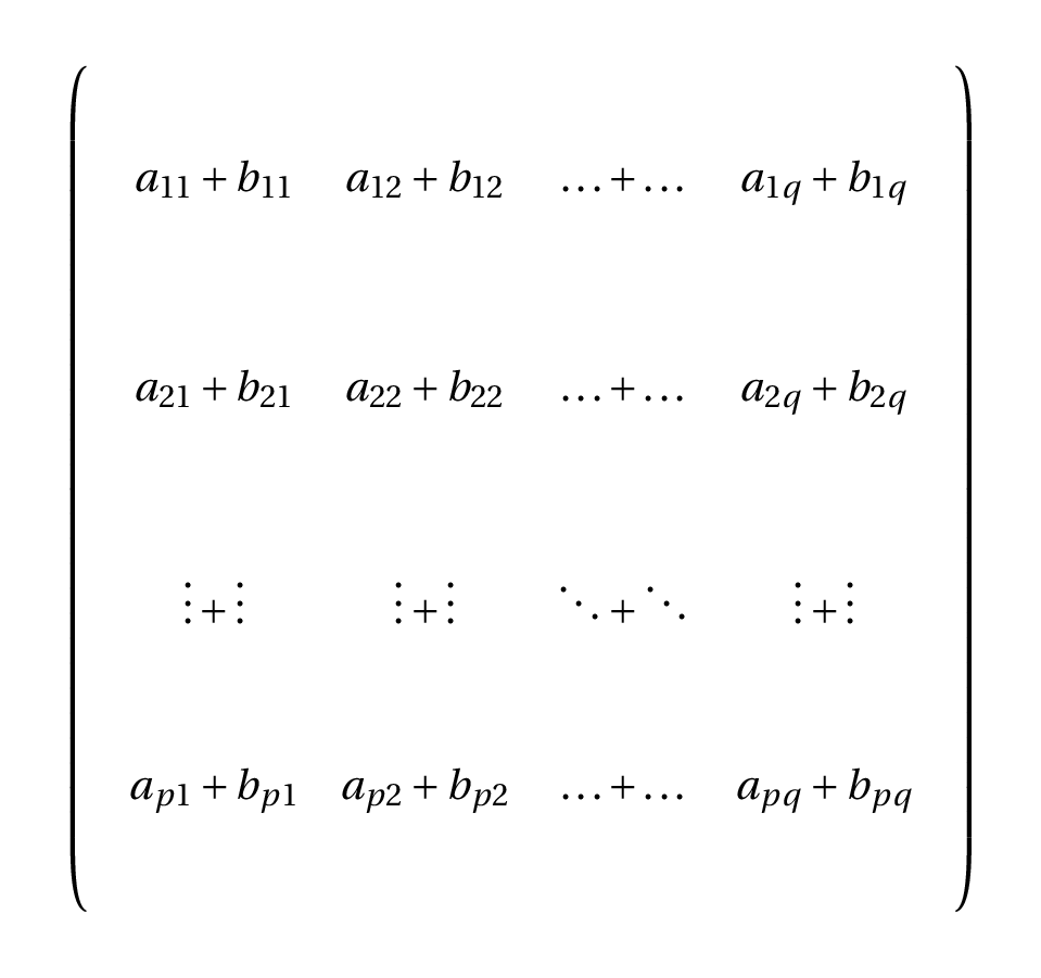
- Adition and subtraction:
- In algebra, we can add or subtract tensors with the same dimensions
- The operation is done element by element


Algebra
Tensor operations
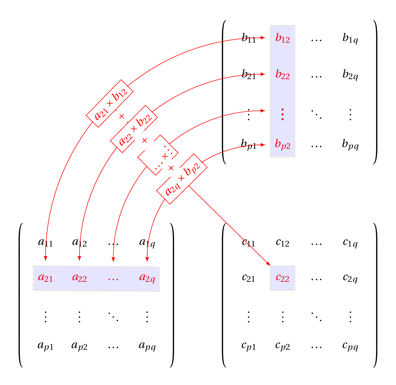
- Matrix multiplication (2D)
- Follows algebra rules: $$\mathbf{C} = \mathbf{AB}$$
$\mathbf{A}$ columns same as $\mathbf{B}$ rows

Algebra
Tensor operations
- Matrix multiplication (2D)
- Follows algebra rules: $$\mathbf{C} = \mathbf{AB}$$
$\mathbf{A}$ columns same as $\mathbf{B}$ rows

Algebra
Tensor operations
- Matrix multiplication (2D)
- Follows algebra rules: $$\mathbf{C} = \mathbf{AB}$$
$\mathbf{A}$ columns same as $\mathbf{B}$ rows

Algebra
Tensor operations
- Matrix multiplication (2D)
- Follows algebra rules: $$\mathbf{C} = \mathbf{AB}$$
$\mathbf{A}$ columns same as $\mathbf{B}$ rows

Algebra
Tensor operations
- Matrix multiplication (2D)
- Follows algebra rules: $$\mathbf{C} = \mathbf{AB}$$
$\mathbf{A}$ columns same as $\mathbf{B}$ rows
Algebra
Tensor operations
- Matrix multiplication (2D)
- Follows algebra rules: $$\mathbf{C} = \mathbf{AB}$$
$\mathbf{A}$ columns same as $\mathbf{B}$ rows

Algebra
Tensor operations
- Matrix multiplication (2D)
- Follows algebra rules: $$\mathbf{C} = \mathbf{AB}$$
$\mathbf{A}$ columns same as $\mathbf{B}$ rows

Algebra
Tensor operations
- Matrix multiplication (2D)
- Follows algebra rules: $$\mathbf{C} = \mathbf{AB}$$
$\mathbf{A}$ columns same as $\mathbf{B}$ rows

Algebra
Tensor operations
- Matrix multiplication (2D)
- Follows algebra rules: $$\mathbf{C} = \mathbf{AB}$$
$\mathbf{A}$ columns same as $\mathbf{B}$ rows

Algebra
- Neuron: linear combination of inputs with non-linear activation

Algebra
Tensor operations
- Tensorflow also allows broadcasting like
numpy - Element-wise operations aligned by the last dimensions


Algebra
Tensor operations
- Tensorflow also allows broadcasting like
numpy - Element-wise operations aligned by the last dimensions
tf.matmul()also works on 3D tensors, in batch- Can be used to compute the product of a batch of 2D matrices
- Example (from Tensorflow
matmuldocumentation):
In : a = tf.constant(np.arange(1, 13, dtype=np.int32), shape=[2, 2, 3])
In : b = tf.constant(np.arange(13, 25, dtype=np.int32), shape=[2, 3, 2])
In : c = tf.matmul(a, b) # or a * b
Out: <tf.Tensor: id=676487, shape=(2, 2, 2), dtype=int32, numpy=
array([[[ 94, 100],
        [229, 244]],

       [[508, 532],
        [697, 730]]], dtype=int32)>
Algebra
Why is this important?
- Our models will be based on this type of operations
- Example batches will be tensors (2D or more)
- Network layers can be matrices of weights (several neurons)
- Loss functions will operate and aggregate on activations and data
In practice mostly hidden
- When we use the
kerasAPI we don't need to worry about this - But it's important to understand how things work
- And necessary to work with basic Tensorflow operations
Training Neural Networks
Basic Example
Basic Example
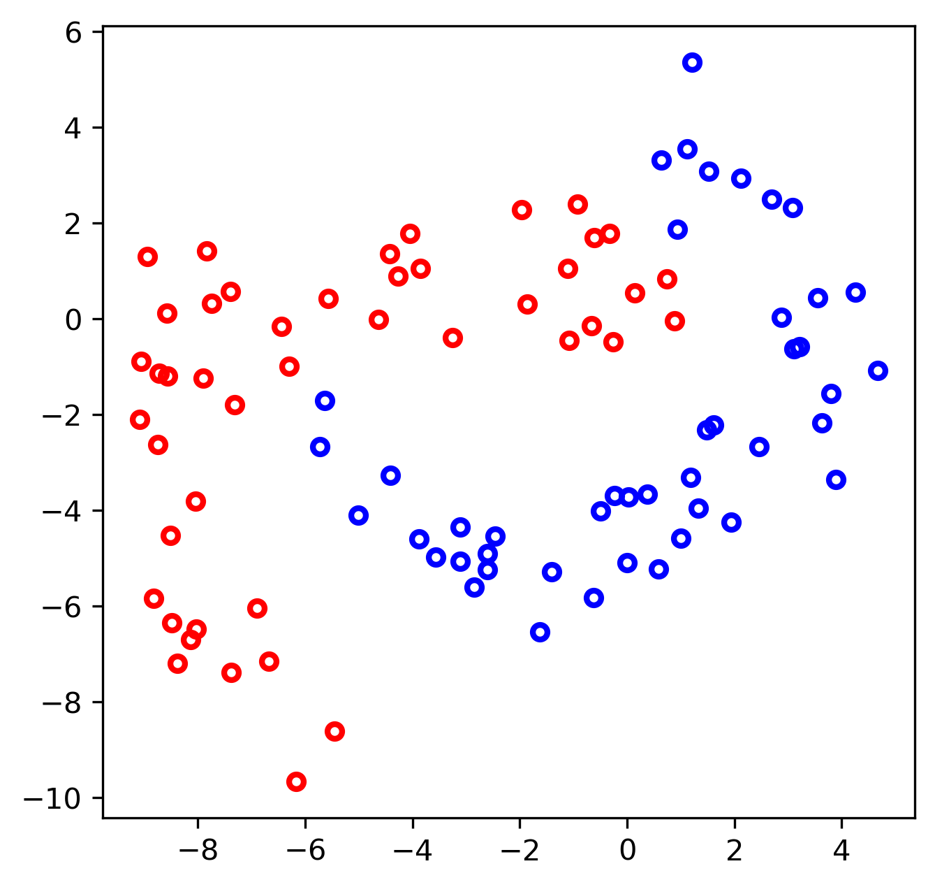
- Classify these data with two weights, sigmoid activation

Basic Example
Computing activation
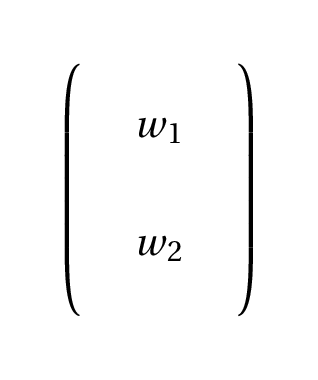
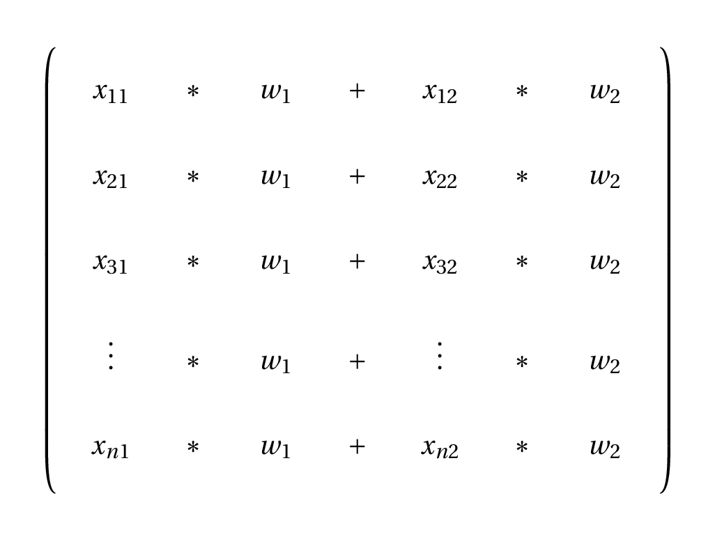
- Input is a matrix with data, two columns for the features, N rows
- To compute $\sum\limits_{j=1}^{2} w_jx_j$ use matrix multiplication

Basic Example
Computing activation
- Input is a matrix with data, two columns for the features, N rows
- To compute $\sum\limits_{j=1}^{2} w_jx_j$ use matrix multiplication
- For each example with 2 features we get one weighted sum
- Then apply sigmoid function, one activation value per example
- Thus, we get activations for a batch of examples
Training Neural Networks
Training (Backpropagation)
Training
Backpropagation
- For weight $m$ on hidden layer $i$, propagate error backwards
- Gradient of error w.r.t. weight of output neuron: $$\frac{\delta E_{kn}^j}{\delta s_{kn}^j} \frac{\delta s_{kn}^j}{\delta net_{kn}^j}\frac{\delta net_{kn}^j}{\delta w_{mkn}}$$
- Chain derivatives through the network: $$\begin{array}{rcl} \Delta w_{min}^j&=& - \eta \left( \sum\limits_{p} \frac{\delta E_{kp}^j}{\delta s_{kp}^j} \frac{\delta s_{kp}^j}{\delta net_{kp}^j}\frac{\delta net_{kp}^j}{\delta s_{in}^j} \right) \frac{\delta s_{in}^j}{\delta net_{in}^j}\frac{\delta net_{in}^j}{\delta w_{min}} \\ \\ &=& \eta (\sum\limits_p \delta_{kp} w_{mkp} ) s_{in}^j(1-s_{in}^j) x_i^j =\eta\delta_{in} x_i^j \end{array}$$
- (See more in lecture notes)
Training
Backpropagation Algorithm
- Propagate the input forward through all layers
- Compute activations
- For output neurons compute
- Loss function
- Derivatives of loss function
- Backpropagate derivatives of loss function to back layers
- Update weights using the computed derivatives
This can be generalized
- Different architectures
- Different activation functions
- Different loss functions, regularization, etc
Training
Computing derivatives
- Symbolic differentiation:
- Compute the expression for the derivatives given the function.
- Difficult, especially with flow control (
if,for)
$$\Delta w_i^j= - \eta \frac{\delta E^j}{\delta w_i} = \eta (t^j - s^j) s^j (1-s^j) x_i^j$$
- Numerical differentiation:
- Use finite steps to compute deltas and approximate derivatives.
- Computationally inefficient and prone to convergence problems.
- Automatic differentiation:
- Apply the chain rule to basic operations that compose complex functions
- product, sum, sine, cosine, etc
- Applicable in general provided we know the derivative of each basic operation
Training
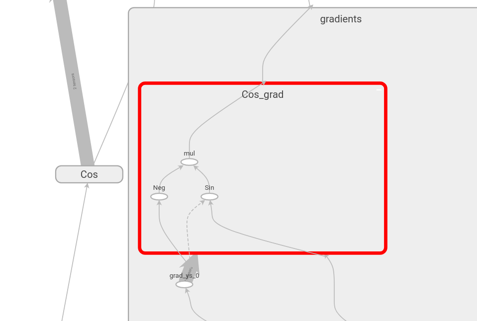
- Automatic differentiation example: $$\underset{x}{\mathrm{argmin}} \left(\cos x \right) \qquad \frac{d \cos x}{dx} = -\sin x$$
Training
- Automatic differentiation example: $$\underset{x}{\mathrm{argmin}} \left(\cos x \right) \qquad \frac{d \cos x}{dx} = -\sin x$$

Training
- Automatic differentiation example: $$\underset{x}{\mathrm{argmin}} \left(x^2 \cos x + \sin x \right) $$
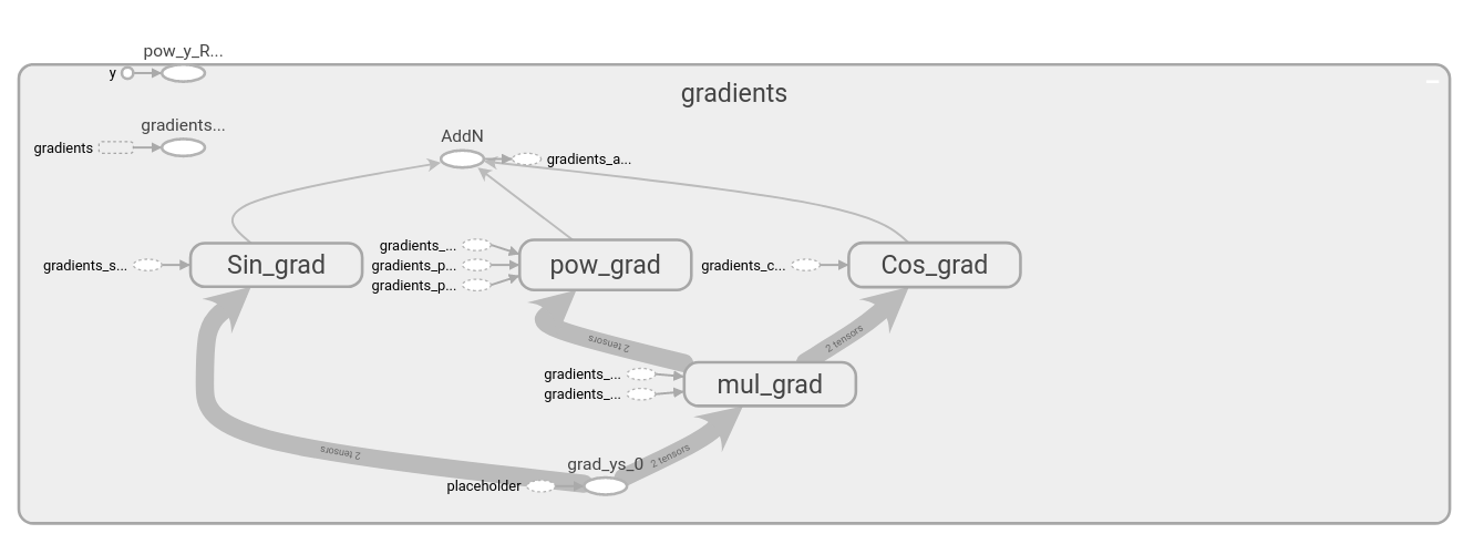
- Tensorflow operators include gradient information
Training
Stochastic Gradient Descent
- Going back to our simple model:


Training
Stochastic Gradient Descent
- Since we can compute the derivatives, we can "slide" down the loss function

Training
Stochastic Gradient Descent
Gradient Descent because of sliding down the gradientStochastic because we are presenting a random minibatch of examples at a time
Training
Stochastic Gradient Descent
Gradient Descent because of sliding down the gradientStochastic because we are presenting a random minibatch of examples at a time
Algorithm:
- Estimate the gradient of $L\left(f\left(x,\theta\right),y\right)$ given $m$ examples: $$\hat{g}_t = \nabla_\theta \left( \frac{1}{m} \sum\limits_{i=1}^{m}L\left(f\left(x^{(i)},\theta\right),y^{(i)}\right)\right)$$
- Update $\theta$ with a learning rate $\epsilon$ $$\theta_{t+1} = \theta_{t} - \epsilon\hat{g}_t$$
Training
SGD can be improved with momentum
- If we are rolling down the surface we could pick up speed
- Use gradients as an "acceleration", with $$v_{t+1} = \alpha v_{t} - \nabla_\theta \left( \frac{1}{m} \sum\limits_{i=1}^{m}L\left(f\left(x^{(i)},\theta\right),y^{(i)}\right)\right)$$
$$\theta_{t+1} = \theta_{t} + \epsilon v_{t+1}$$
Training
SGD can be improved with momentum
- SGD
- SGD + 0.9 momentum
Training
Minibatch size
- Averaging over a set of examples gives a (slightly) better estimate of the gradient, improving convergence
- (Note that the true gradient is for the mean loss over all points)
- The main advantage of batches is in using multicore hardware (GPU, for example)
- This is also the reason for power of 2 minibatch sizes (8, 16, 32, ...)
- Smaller minibatches improve generalization because of the random error
- The best for this is a minibatch of 1, but this takes much longer to train
- In practice, minibatch size will probably be limited by RAM.
Training
- Minibatch of 10
- Minibatch of 1
- Note: the actual time is much longer for minibatch of 1
Training Neural Networks
Improving the model
Better Models
Our simple (pseudo) neuron lacks a bias
$$y = \sum\limits_{j=1}^{2} w_jx_j + bias$$

Better Models
Our simple (pseudo) neuron lacks a bias
- This means that it is stuck a (0,0)
- No bias input
- With bias input
Better Models
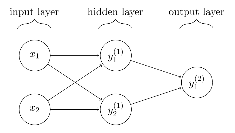
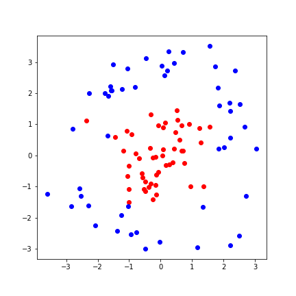
And one neuron cannot properly separate these sets
- We need a better model:

Better Models
Neural Networks stack nonlinear transformations


Training Neural Networks
Other Details
Other Details
Initialization
- Weights: random values close to zero (Gaussian or uniform p.d)
- Need to break symmetry between neurons (but bias can start the same)
- Some activations (e.g. sigmoid) saturate rapidly away from zero

- (There are other, more sophisticated methods)
Other Details
Convergence
- Since weight initialization and order of examples is random, expect different runs to converge at different epochs

Other Details
Convergence
- Standardize the inputs: $x_{new} = \frac{x -\mu(X)}{\sigma(X)}$
- It is best to avoid different features weighing differentely
- It is also best to avoid very large or very small values due to numerical problems
- Shifting the mean of the inputs to 0 and scaling the different dimensions also improves the loss function "landscape"

Other Details
Training schedules
- Epoch: one full pass through the training data
- Mini-batch: one batch with part of the training data
Generally needs many epochs to train
- (the greater the data set, the fewer the epochs, other things being equal)
Other Details
Shuffle the data in each epoch
- Otherwise some patterns will repeat
Other Details
Take care with the learning rate
- Too small and training takes too long
- But if it is too large convergence is poor at the end
Training Neural Networks
Tutorial: Keras Sequential API
Keras Sequential
Building a model with Keras
import numpy as np
from tensorflow.keras.optimizers import SGD
from tensorflow.keras.models import Sequential
from tensorflow.keras.layers import Dense
from t01_aux import plot_model   #auxiliary plotting function
- Create a
Sequentialmodel and add layers
model = Sequential()
model.add(Dense(4, activation = 'sigmoid',input_shape=(inputs,)))
- In this tutorial,
inputsis 2 for the 2D dataset, but it can vary
model.add(Dense(4, activation = 'sigmoid'))
model.add(Dense(1, activation = 'sigmoid'))
- Only the first layer of a dense network needs the input size
Keras Sequential
- Compile and check the model
opt = SGD(lr=INIT_LR, momentum=0.9)
model.compile(loss="mse", optimizer=opt,	metrics=["mse"])
model.summary()
_________________________________________________________________
Layer (type)                 Output Shape              Param #
=================================================================
dense (Dense)                (None, 4)                 12
_________________________________________________________________
dense_01 (Dense)             (None, 4)                 20
_________________________________________________________________
dense_02 (Dense)             (None, 1)                 5
=================================================================
Total params: 37
Trainable params: 37
Non-trainable params: 0
_________________________________________________________________
Keras Sequential
- Now we can train the model and obtain the history of training.
- We can also plot the loss function and how the model classifies:
H = model.fit(X, Y, batch_size=16, epochs=10000)
plt.plot(H.history['loss'])
plot_model(model,X,Y)


Training Neural Networks
Summary
Training Neural Networks
Summary
- Matrix algebra
- Automatic Differentiation
- Layers and nonlinear transformations
- Training multilayer feedforward neural networks
- MLP is a special case, fully connected
Further reading:
- Goodfellow, chapters 2 (algebra), 4 (calculus) and 8 (optimization)
- Andrej Karpathy's Intro to NNs and backprop: https://www.youtube.com/watch?v=VMj-3S1tku0