Técnicas de IA para Biologia
4 - Convolutional Networks
André Lamúrias
Convolutional Networks
Summary
- What is convolution
- Convolution layers and neural networks (CNNs)
- Pooling
- Classification with convolutional networks
- CNN tutorial: Fashion MNIST classification with CNN and Keras
Convolutional Networks
Convolution
Convolution
Definition:
- Integral of the product of two functions, one of which was shifted and inverted $$(f*g)(t) = \int_{-\infty}^{\infty} f(\tau) g(t-\tau) d\tau = \int_{-\infty}^{\infty} f(t-\tau) g(\tau) d\tau$$
- Used in many applications, such as probabilities or linear time-invariant systems
Convolution
$$(f*g)(t) = \int_{-\infty}^{\infty} f(\tau) g(t-\tau) d\tau = \int_{-\infty}^{\infty} f(t-\tau) g(\tau) d\tau$$- Intuition: Suppose a LTIS with this response:

Convolution
$$(f*g)(t) = \int_{-\infty}^{\infty} f(\tau) g(t-\tau) d\tau = \int_{-\infty}^{\infty} f(t-\tau) g(\tau) d\tau$$- Subject to this impulse

- How do we compute the output?
Convolution
$$(f*g)(t) = \int_{-\infty}^{\infty} f(\tau) g(t-\tau) d\tau = \int_{-\infty}^{\infty} f(t-\tau) g(\tau) d\tau$$- First we take the symmetric of the response:

- How do we compute the response?
Convolution
$$(f*g)(t) = \int_{-\infty}^{\infty} f(\tau) g(t-\tau) d\tau = \int_{-\infty}^{\infty} f(t-\tau) g(\tau) d\tau$$- Now we integrate product at different time shifts
Convolution
For finding patterns
- Suppose we have this signal and want to detect the spike pattern

Convolution
For finding patterns
- We create this "detector" function (inverted)

Convolution
$$(f*g)(t) = \int_{-\infty}^{\infty} f(\tau) g(t-\tau) d\tau = \int_{-\infty}^{\infty} f(t-\tau) g(\tau) d\tau$$- We detect the pattern integrating at different time shifts
Convolution
Motivation:
- Use a kernel (w) to modify the input (x) and create a new function (s) using weighted values "around" the input
- E.g. a weighted average of most recent values in a time series, local features of an image, etc, $$s(t) = (x*w)(t) = \sum_{m=-\infty}^{\infty} x(t) w(t-m) $$
- In practice, for CNN:
- The input is a finite, discrete set of values (assumed 0 everywhere else)
- The kernel is a finite set of parameters that will be learned
- The output will be tensor, typically of the same size and shape as the input
Convolution
Two-dimensional convolution
- We often use convolution in more than one dimension (e.g. for images) $$S(i,j) = (I*K)(i,j) = \sum_{m}\sum_{n} I(m,n) K(i-m,j-n) $$
- Since convolution is commutative, we often use: $$S(i,j) = (I*K)(i,j) = \sum_{m}\sum_{n} I(i-m,j-n) K(m,n)$$
- I.e. we index the kernel and the image around (i,j)
Convolutional networks
CNN
CNN
Motivation for convolutional networks
- Sparse interactions (sparse connectivity or sparse weights)
- Since the kernel is smaller than the input, we need fewer parameters
- Shared parameters
- Connections are sparse but the same parameters are used over all inputs
- Equivariance
- Convolutions are equivariant to some transformations
- I.e. applying the transformation (e.g. translation) to the input is the same as applying it to the convolution
CNN
Motivation: sparse interactions
- Convolutional networks have fewer connections than MLP

Goodfellow, Bengio, Courville, Deep Learning 2016
CNN
Motivation: sparse interactions
- Convolutional networks have fewer connections than MLP
- But deeper neurons can still have a large receptive field in the input

Goodfellow, Bengio, Courville, Deep Learning 2016
CNN
Motivation: parameter sharing
- The same parameter is used for many inputs
- E.g. edge detection by subtracting pixel on the left

Goodfellow, Bengio, Courville, Deep Learning 2016
CNN
Motivation: equivariance
- Moving the input image is equivalent to moving the output of the convolution filter (the feature map)

Goodfellow, Bengio, Courville, Deep Learning 2016
CNN
Receptive field and multiple filters
- Visual cortex neurons respond to a small receptive field in retina
- Neurons in convolution layers have this property
- Multiple convolution filters are generally applied


Images: Aphex34, CC-SA; UFLDL tutorial, Stanford (Ng et. al.)
CNN
Receptive field and multiple filters
- Multiple convolution filters are generally applied
- We generally represent convolution layers as 3D volumes of neurons (in image processing), stacking the different convolution filters

Image: CS231n Stanford (Fei-Fei Li et. al.)
CNN
Nonlinear tranformation
- A convolution is a linear transformation, so in CNN the convolution filter generally feeds into a nonlinear response (usually ReLU)


CNN
Hyperparameters of a convolution layer
- Depth: the number of filters being learned
- Stride: How the receptive field "jumps"
- Padding: to prevent output from shrinking


Image: Machine learning guru, http://machinelearninguru.com
CNN
Example: convolution network
- Stanford (CS231, Fei-Fei Li et. al.)
- http://cs231n.github.io/convolutional-networks/

Convolutional networks
Pooling
Pooling
Typical architecture of a convolutional layer
- Convolutions: several convolutions in parallel, generating a set of linear activations
- Nonlinear activation: applied to each linear output (typically ReLU)
- (detector stage)
- Pooling: aggregates the outputs in a single output for each region
Pooling
Pooling: aggregating outputs
- Example: max pooling

Image: Aphex34, CC-SA
Pooling
Pooling: aggregating outputs
- Typical pooling functions:
- Max pooling, average pooling, L$^2$ norm pooling: $\sqrt{ \sum x_i^2}$
- Pooling makes model nearly invariant to small shifts in input
Pooling Stride
- We may want to regulate the overlap of pooling regions
- If the stride is equal to the size of the regions, then there is no overlap
- Stride also reduces the dimension
- (pooling of stride 1, with padding, preserves dimension)
Classificaton with CNN
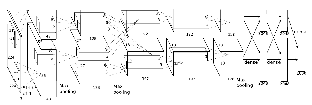
For classification, conv layers combined with MLP
- Fully connected layers at the end to predict class for example
- Forces fixed-sized input and output not spacial

Alex Krizhevsky, Ilya Sutskever, Geoffrey E. Hinton, 2012
Convolutional networks
Tutorial: Keras Sequential API
Keras Sequential
Building a model with Keras
- Start by importing classes:
from tensorflow.keras.optimizers import SGD
from tensorflow.keras.models import Sequential
from tensorflow.keras.layers import BatchNormalization,Conv2D,MaxPooling2D,
from tensorflow.keras.layers import Activation, Flatten, Dropout, Dense
Keras Sequential
Building a model with Keras
- Create a
Sequentialmodel and add layers
model = Sequential()
model.add(Conv2D(32, (3, 3), padding="same", input_shape=(28,28,1)))
model.add(Activation("relu"))
...
model.add(MaxPooling2D(pool_size=(2, 2)))
model.add(Conv2D(64, (3, 3), padding="same"))
...
model.add(Flatten())
model.add(Dense(512))
model.add(Activation("relu"))
model.add(BatchNormalization())
model.add(Dropout(0.5))
model.add(Dense(10))
model.add(Activation("softmax"))
Keras Sequential
Side note:
- (Current consensus, but some opinions may vary)
- Use batch normalization after activation so that input of following layer is standardized
- Use dropout after all batch normalizations
- Otherwise you may need to compensate the rescaling of dropout when shifting to prediction mode
- Dropout may have some benefits in convolution layers but in that case it is not the same as dropout in dense layers
Keras Sequential
Compiling the model
opt = SGD(lr=INIT_LR, momentum=0.9, decay=INIT_LR / NUM_EPOCHS)
model = create_model()
model.compile(loss="categorical_crossentropy", optimizer=opt,
	metrics=["accuracy"])
- Now we can train the model and save the weights.
history = model.fit(trainX, trainY, validation_data=(testX, testY),
                  batch_size=BS, epochs=NUM_EPOCHS)
model.save_weights('fashion_model.weights.h5')
- The saved weights can be loaded with
model.load_weights(file_name)
Keras Sequential
Monitoring
- The
fitmethod returns a history object (parameters, model, etc)
history = model.fit(trainX, trainY, validation_data=(testX, testY),
                    batch_size=BS, epochs=NUM_EPOCHS)
In: history.history
Out:
 {'acc': [0.7736167, ...],
  'loss': [0.6834171069622039, ...],
  'val_acc': [0.1974, ...],
  'val_loss': [2.1077217151641845, ...]}
Convolutional networks
Tutorial: Regression and CNN
Tutorial
Regression with the Auto MPG Data Set
- Predict the fuel consumption of cars
- Auto MPG Data Set, available at the UCI repository
- Some pointers:
- Shuffle the data before splitting into training and validation sets
- Target: first column, MPG (miles per gallon)
- Standardize features and target value
- Standardizing target centers the output and minimizes numerical problems
- Only 392 examples. Use 300 for training and 92 for validation.
- Linear output for the last neuron (only one neuron)
- Mean squared error loss function for training
- Try different activations and learning parameters (rate, momentum)
Tutorial
Regression with the Auto MPG Data Set
- Load, standardize, use 300 for train and rest for validation:
data = np.loadtxt('AutoMPG.tsv',skiprows=1)
np.random.shuffle(data)
means = np.mean(data,axis=0)
stds = np.std(data,axis=0)
data = (data-means)/stds

valid_Y = data[300:,0]
valid_X = data[300:,1:]

Y = data[:300,0]
X = data[:300,1:]
Tutorial
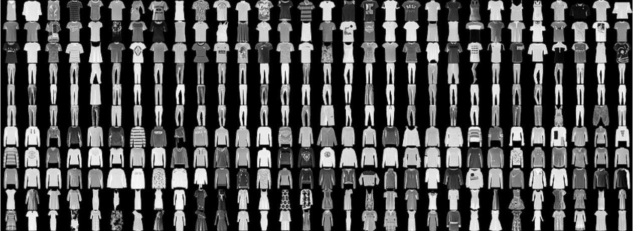
Fashion MNIST
https://github.com/zalandoresearch/fashion-mnist
- Grayscale images, 28x28, 10 classes of clothing

Tutorial
Import the dataset and set up the data
from tensorflow import keras
((trainX, trainY), (testX, testY)) = keras.datasets.fashion_mnist.load_data()
trainX = trainX.reshape((trainX.shape[0], 28, 28, 1))
testX = testX.reshape((testX.shape[0], 28, 28, 1))
trainX = trainX.astype("float32") / 255.0
testX = testX.astype("float32") / 255.0
# one-hot encode the training and testing labels
trainY = keras.utils.to_categorical(trainY, 10)
testY = keras.utils.to_categorical(testY, 10)
- One-hot encoding for encoding multi-class.
[[0. 0. 0. 0. 0. 1. 0. 0. 0. 0.]
 [0. 0. 0. 0. 0. 0. 0. 0. 1. 0.]
...
- Softmax will output vectors with sum of 1 and with probabilities of belonging to each class
Tutorial
Model for this exercise:
- First stack:
- Two convolution layers with $3\times3$ kernel, padding "same", 32 filters, ReLU activation and batch normalization
- Max pooling of size $2\times2$ and same stride
- Optional: you can try adding dropout layer with 25% dropout probability (but results seem to be worse)
- Second stack: Identical to first but with 64 filters
- Dense layer of 512 neurons with ReLU activation, batch normalization and dropout of 50%
- Softmax layer with 10 neurons.
- Use the SGD optimizer and about 25 epochs, save after fitting
- Optional: Experiment changing the model and optimizers
Convolutional networks
Summary
Convolutional networks
Summary
- Convolutions
- Convolution layers
- Classification with convolutional networks
- CNN tutorial using the Keras sequential API
Further reading:
- Goodfellow et.al, Deep learning, Chapter 9
- Tensorflow Keras API
- https://www.tensorflow.org/guide/keras